1
2
3
4
5
6
7
8
9
10
11
12
13
14
15
16
17
18
19
20
21
22
23
24
25
26
27
28
29
30
31
32
33
34
35
36
37
38
39
40
41
42
43
44
45
46
47
48
49
50
| #!/usr/bin/env python3
import seaborn as sns
import numpy as np
import pandas as pd
import matplotlib.pyplot as plt
sns.set(color_codes=True)
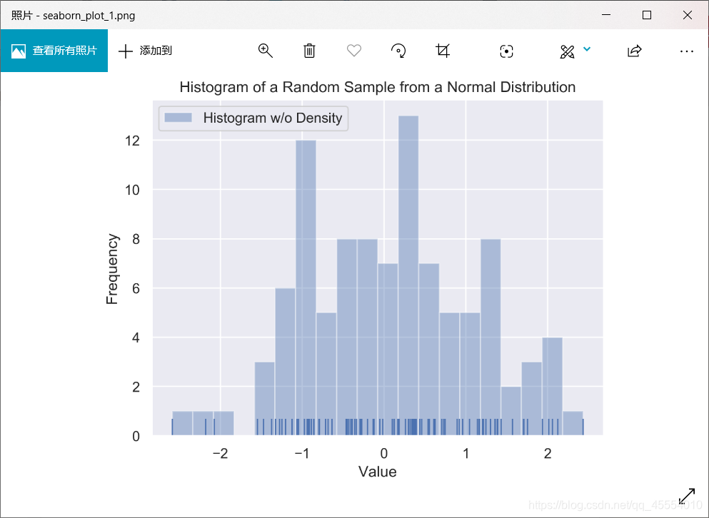
# 直方图
x = np.random.normal(size=100)
sns.distplot(x, bins=20, kde=False, rug=True, label="Histogram w/o Density")
sns.utils.axlabel("Value", "Frequency")
plt.title("Histogram of a Random Sample from a Normal Distribution")
plt.legend()
plt.savefig("seaborn_plot_1.png", dpi=400, bbox_inches='tight')
plt.show()
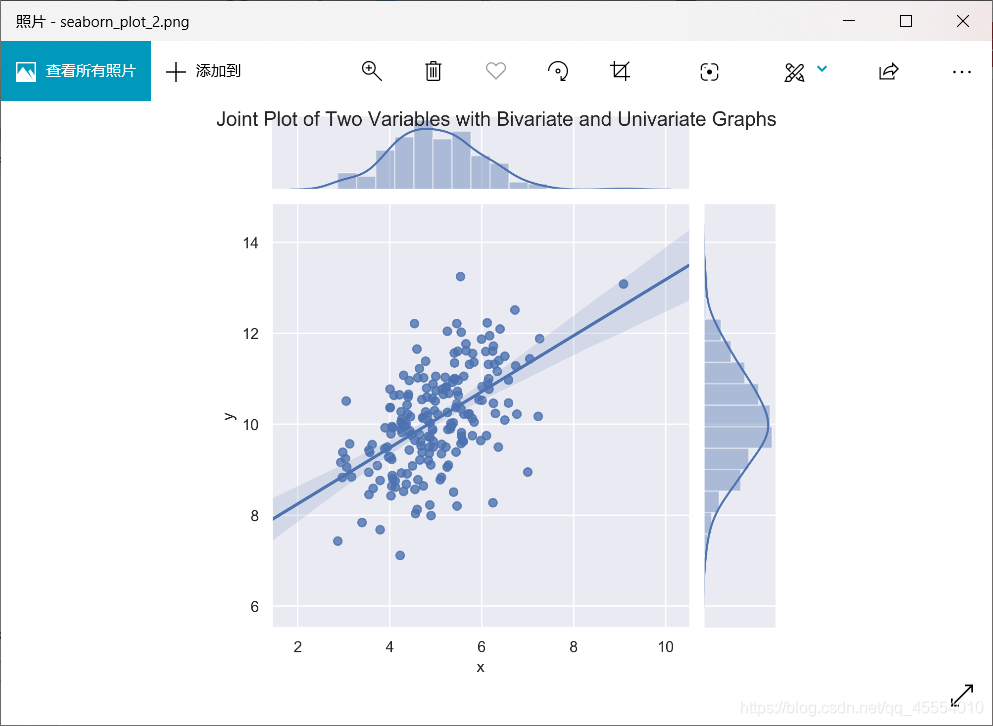
# 带有回归直线的散点图与单变量直方图
mean, cov = [5, 10], [(1, .5), (.5, 1)]
data = np.random.multivariate_normal(mean, cov, 200)
data_frame = pd.DataFrame(data, columns=["x", "y"])
sns.jointplot(x="x", y="y", data=data_frame, kind="reg").set_axis_labels("x", "y")
plt.suptitle("Joint Plot of Two Variables with Bivariate and Univariate Graphs")
plt.savefig("seaborn_plot_2.png", dpi=400, bbox_inches='tight')
plt.show()
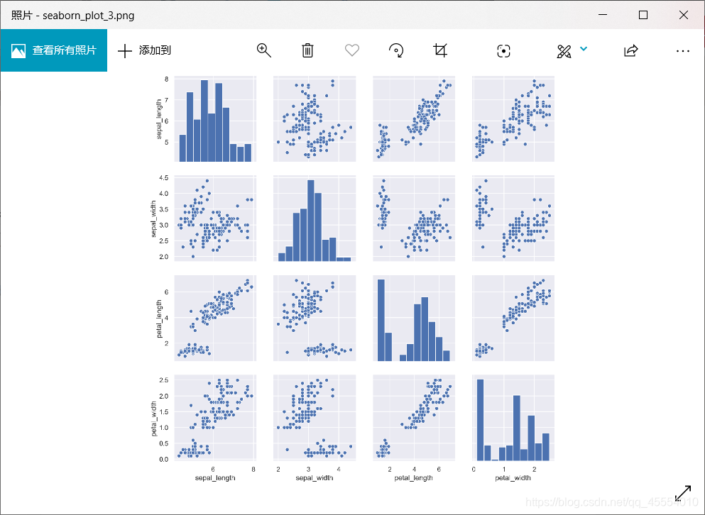
# 成对变量之间的散点图与单变量直方图
iris = sns.load_dataset("iris")
sns.pairplot(iris)
plt.savefig("seaborn_plot_3.png", dpi=400, bbox_inches='tight')
plt.show()
# 按照某几个变量生成的箱线图
tips = sns.load_dataset("tips")
sns.catplot(x="time", y="total_bill", hue="smoker", col="day", data=tips, kind="box", height=4, aspect=.5)
plt.savefig("seaborn_plot_4.png", dpi=400, bbox_inches='tight')
plt.show()
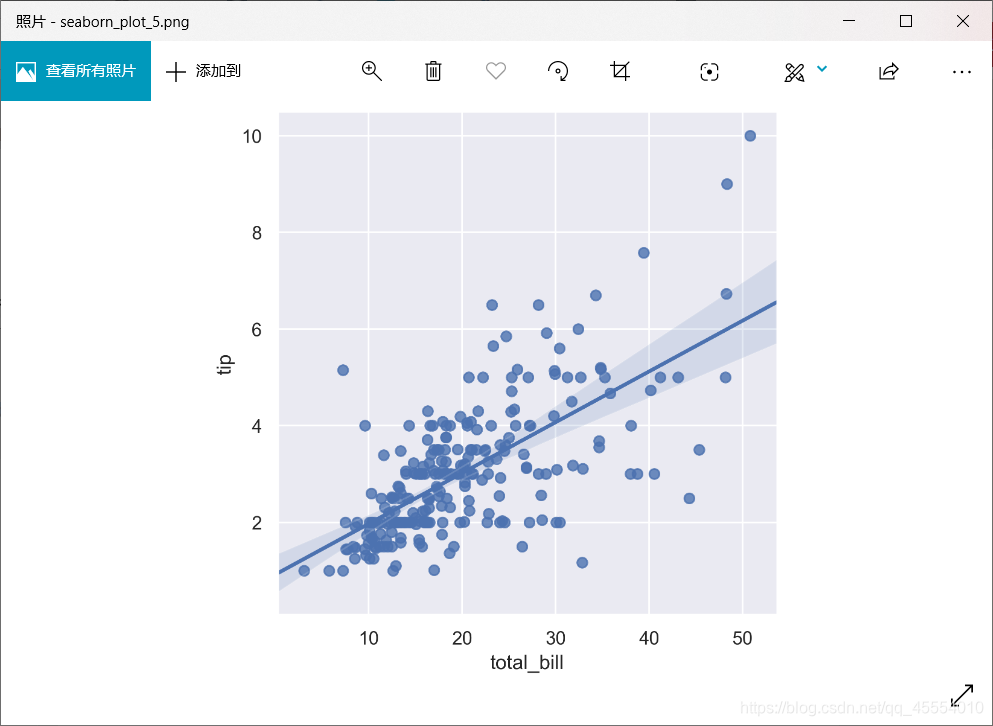
# 带有bootstrap置信区间的线性回归模型
sns.lmplot(x="total_bill", y="tip", data=tips)
plt.savefig("seaborn_plot_5.png", dpi=400, bbox_inches='tight')
plt.show()
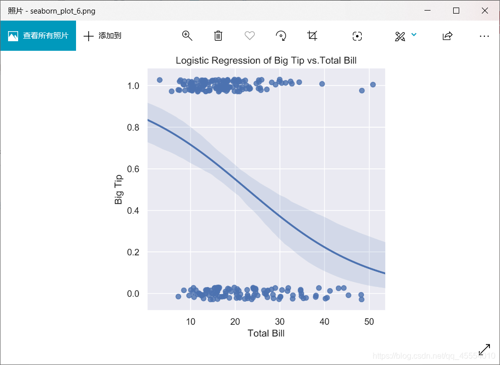
# 带有bootstrap置信区间的逻辑斯蒂回归模型
tips["big_tip"] = (tips.tip / tips.total_bill) > .15
sns.lmplot(x="total_bill", y="big_tip", data=tips, logistic=True, y_jitter=.03).set_axis_labels("Total Bill", "Big Tip")
plt.title("Logistic Regression of Big Tip vs.Total Bill")
plt.savefig("seaborn_plot_6.png", dpi=400, bbox_inches='tight')
plt.show()
|
 )
) )
) )
) )
) )
)